class: center, middle, inverse, title-slide .title[ # Chapter 7 move beyond linear ] .author[ ### Chun Su ] .institute[ ### R-ladies Philly ] .date[ ### 2022-09-13 ] --- ## The extensions of linear models - Polynomial regression - Step function - Splines - polynomial splines - natural splines - smoothing splines - Local regression - Generalized Additive Model (GAM) --- ## Polynomial regression - raising each of the original predictors to a power  - Generally speaking, it is unusual to use greater than 3 or 4 because for large values of X the polynomial curve can become overly flexible and can take on some very strange shapes. ```r lm(wage ~ poly(age, 4, raw = T), data = Wage) ``` --- ## Step functions - K points break X into bins (K + 1), then fit different **constant** (**indicator function**) in each bin. Indicator function equals 0 or 1, and only one 1 cross K+1 functions.  ```r lm(wage ∼ cut(age, 4), data = Wage) ``` -- ### Basic function  --- ## Regression splines - Piecewise Polynomials: - **knots** divide to different regions of X - **degree of polynomials** fit for each region. -- - polynomial spline (`splines::bs`) - piecewise polynomial with contraints on knots - three constraints (continuity, continuity of the first derivative, and continuity of the second derivative) - **degrees of freedom** = number_of_knots + degree_of_polynomials + number_of_intercept - in practice it is common to place knots at uniform quantiles of the data. -- - natural spline (`splines::ns`) - polynomial spline with additional boundary constraints - **degrees of freedom** = number_of_knots + 1 + number_of_intercept - usually degree of polynomials = 3 - `lm(wage ∼ ns(age, df = 4), data = Wage)` using least squares to estimate the spline coefficients ??? https://stats.stackexchange.com/questions/517375/splines-relationship-of-knots-degree-and-degrees-of-freedom --- ## smoothing spline (`smooth.spline`) - a function g that makes RSS small, but that is also smooth - "Loss+Penalty"  - The first derivative g′(t) measures the slope of a function at t - the second derivative g''(t) is a measure of its roughness - the function g(x) that minimizes (7.11) is a shrunken natural cubic spline with knots at x1, . . . , xn. - **effective degrees of freedom** (df_lambda) decrease from n to 2 when lambda increase from 0 to inf ```r fit <- smooth.spline(age, wage, df = 16) ``` --- ## local regression (`stats::loess`) - fit at a target point x0 using only the regression nearby training observations - Hyperparameter **span s** is the proportion of points used to compute the local regression at x0 - The smaller the value of s, the more local and wiggly will be our fit - `s = k/n` where k is k nearest neighbors. - Using a **weighted** least squares regression ```r fit <- loess(wage ∼ age, span = .2, data = Wage) ``` --- ## Generalized additive models (GAMs) - provide a general framework for generalized extending a standard linear model by allowing non-linear functions of each additive of the variables,while maintaining additivity. - a big linear regression model using an appropriate choice of basis functions ```r gam1 <- lm(wage ~ ns(year, 4) + ns(age, 5) + education, data = Wage) gam.s <- gam(wage ~ gam::s(age, df = 16) + education, data = Wage) gam.lo <- gam(wage ~ gam::l(age, span = 0.7) + education, data = Wage) ``` --- ## budget data ```r library(tidymodels) library(ISLR) Wage <- as_tibble(Wage) # initial split set.seed(123) wage_split <- initial_split(Wage) wage_train <- training(wage_split) wage_test <- testing(wage_split) # cv folds set.seed(234) wage_folds <- vfold_cv(wage_train) ``` --- ## polynomial regression tune The order of polynomial is defined by `recipe::step_poly` at feature engineer step. ```r # recipe rec_poly <- recipe(wage ~ age, data = wage_train) %>% step_poly(age, degree = tune(), options = list(raw = TRUE)) # model lm_spec <- linear_reg() %>% set_mode("regression") %>% set_engine("lm") # workflow poly_wf <- workflow() %>% add_model(lm_spec) %>% add_recipe(rec_poly) # specify hyperparameter tune degree_grid <- tibble(degree = 1:5) # tune poly_rs <- poly_wf %>% tune_grid( resamples = wage_folds, grid = degree_grid ) ``` --- ## select best degree of polynomial 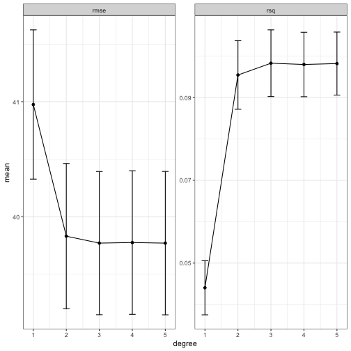<!-- --> --- ## last fit using best degree of polynomial ```r best_hyper <- select_by_one_std_err(poly_rs, metric = "rmse", degree) best_hyper ``` ``` ## # A tibble: 1 × 9 ## degree .metric .estimator mean n std_err .config .best .bound ## <int> <chr> <chr> <dbl> <int> <dbl> <chr> <dbl> <dbl> ## 1 2 rmse standard 39.8 10 0.631 Preprocessor2_Model1 39.8 40.4 ``` ```r poly_wf_final <- poly_wf %>% finalize_workflow(best_hyper) %>% last_fit(wage_split) poly_wf_final %>% extract_workflow() %>% saveRDS("wage_poly_model.rds") ``` --- ## final model metrics and parameters - metrics on test data ```r poly_wf_final %>% collect_metrics() ``` ``` ## # A tibble: 2 × 4 ## .metric .estimator .estimate .config ## <chr> <chr> <dbl> <chr> ## 1 rmse standard 40.4 Preprocessor1_Model1 ## 2 rsq standard 0.0495 Preprocessor1_Model1 ``` - check co-efficient ```r poly_wf_final %>% extract_fit_parsnip() %>% tidy() ``` ``` ## # A tibble: 3 × 5 ## term estimate std.error statistic p.value ## <chr> <dbl> <dbl> <dbl> <dbl> ## 1 (Intercept) -18.2 9.23 -1.98 4.82e- 2 ## 2 age_poly_1 5.70 0.439 13.0 2.74e-37 ## 3 age_poly_2 -0.0574 0.00500 -11.5 9.72e-30 ``` --- ## prediction using finalized polynomial 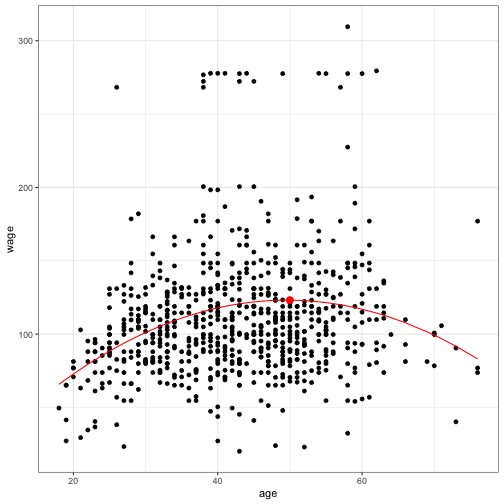<!-- --> ```r trained_poly_wf <- readRDS("wage_poly_model.rds") trained_poly_wf %>% augment(new_data =data.frame(age = 50)) ``` ``` ## # A tibble: 1 × 2 ## age .pred ## <dbl> <dbl> ## 1 50 123. ``` --- ## step function `step_discretize()` will convert a numeric variable into a factor variable with n bins, n here is specified with `num_breaks` If you already know where you want the step function to break then you can use `step_cut()` and supply the `breaks` manually. ```r rec_discretize <- recipe(wage ~ age, data = Wage) %>% step_discretize(age, num_breaks = 4) discretize_wf <- workflow() %>% add_model(lm_spec) %>% add_recipe(rec_discretize) discretize_rs <- fit_resamples( discretize_wf, resamples = wage_folds ) discretize_rs %>% collect_metrics() ``` ``` ## # A tibble: 2 × 6 ## .metric .estimator mean n std_err .config ## <chr> <chr> <dbl> <int> <dbl> <chr> ## 1 rmse standard 40.5 10 0.681 Preprocessor1_Model1 ## 2 rsq standard 0.0694 10 0.00956 Preprocessor1_Model1 ``` ??? `fit_resamples` their only purpose is for computing the .metrics to estimate performance. --- ## step function final fit ```r discretize_wf_final <- discretize_wf %>% last_fit(wage_split) discretize_wf_final %>% extract_fit_parsnip() %>% tidy() ``` ``` ## # A tibble: 4 × 5 ## term estimate std.error statistic p.value ## <chr> <dbl> <dbl> <dbl> <dbl> ## 1 (Intercept) 93.5 1.69 55.2 0 ## 2 agebin2 24.2 2.39 10.1 1.34e-23 ## 3 agebin3 28.2 2.36 12.0 4.46e-32 ## 4 agebin4 22.4 2.47 9.08 2.23e-19 ``` --- ## step function prediction 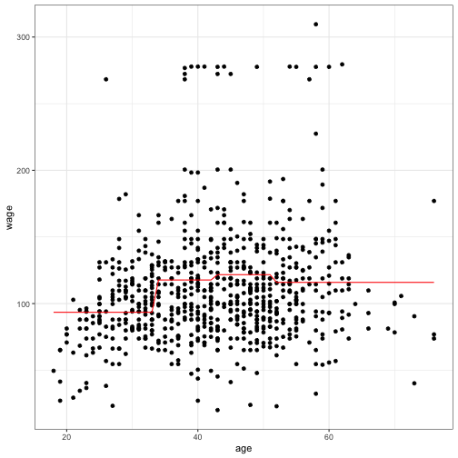<!-- --> --- ## polynomial splines / cubic splines In the example, author directly specifies the internal breakpoints that define the spline, which usually takes quantiles for multiple knots. Here, we tune number of `knots` by degree of freedom `deg_free`. For more details, `?step_bs` or `?bs`. ```r rec_cubic <- recipe(wage ~ age, data = Wage) %>% step_bs(age, deg_free = tune(), degree = 3) cubic_wf <- workflow() %>% add_model(lm_spec) %>% add_recipe(rec_cubic) grid_df <- grid_regular( deg_free(range = c(4,12)), levels = 5 ) cubic_rs <- tune_grid( cubic_wf, resamples = wage_folds, grid = grid_df ) ``` --- ## select best hyparameter (`deg_free`) ```r best_hyper <- select_by_one_std_err(cubic_rs, metric = "rmse", deg_free) best_hyper ``` ``` ## # A tibble: 1 × 9 ## deg_free .metric .estimator mean n std_err .config .best .bound ## <int> <chr> <chr> <dbl> <int> <dbl> <chr> <dbl> <dbl> ## 1 4 rmse standard 39.8 10 0.625 Preprocessor1_Model1 39.8 40.4 ``` ```r cubic_wf_final <- cubic_wf %>% finalize_workflow(best_hyper) %>% last_fit(wage_split) ``` --- ## final model metrics and parameters - metrics on test data ```r cubic_wf_final %>% collect_metrics() ``` ``` ## # A tibble: 2 × 4 ## .metric .estimator .estimate .config ## <chr> <chr> <dbl> <chr> ## 1 rmse standard 40.3 Preprocessor1_Model1 ## 2 rsq standard 0.0527 Preprocessor1_Model1 ``` - check co-efficient ```r cubic_wf_final %>% extract_fit_parsnip() %>% tidy() ``` ``` ## # A tibble: 5 × 5 ## term estimate std.error statistic p.value ## <chr> <dbl> <dbl> <dbl> <dbl> ## 1 (Intercept) 54.5 6.01 9.06 2.78e-19 ## 2 age_bs_1 46.6 9.81 4.75 2.12e- 6 ## 3 age_bs_2 84.8 7.28 11.7 1.64e-30 ## 4 age_bs_3 53.8 11.9 4.53 6.19e- 6 ## 5 age_bs_4 37.3 13.9 2.68 7.49e- 3 ``` --- ## Compare predictions among multiple models. .pull-left[ 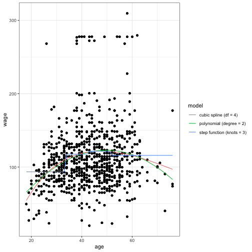<!-- --> ] .pull-right[ 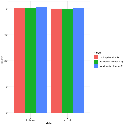<!-- --> ]