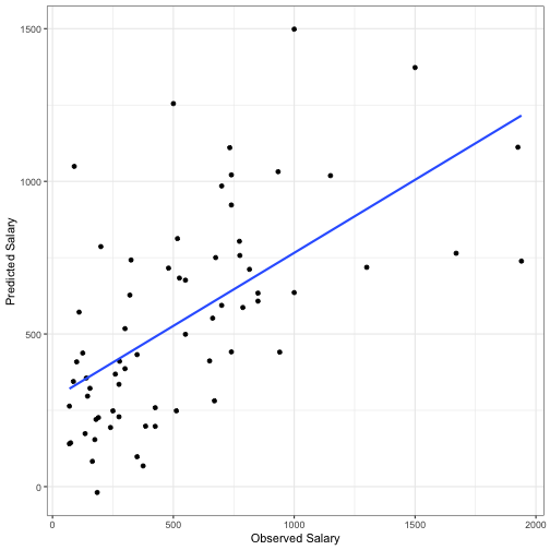
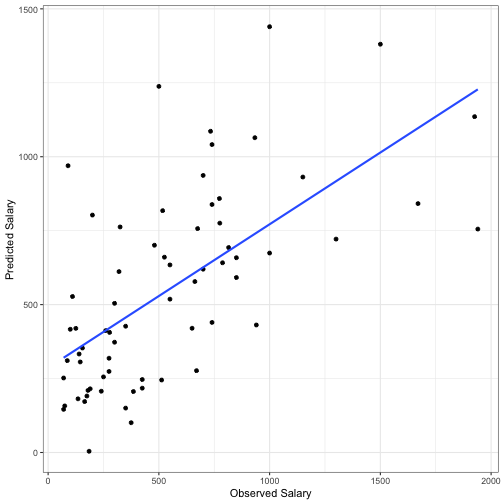
Chapter 6 Linear model selection and regularization

class: center, middle, inverse, title-slide

.title[
# Chapter 6 Linear model selection and regularization
]
.author[
### Chun Su
]
.institute[
### R-ladies Philly
]
.date[
### 2022-08-18
]

---

## Alternative fitting procedures to OLS

#### Why?
- prediction accuracy (p > n)

- shrink the estimated coefficients to reduce the variance at the cost of a negligible increase in bias.

- model interpretability

- automatic feature selection by setting coefficients to 0

#### How?

- subset selection

- shrinkage/regularization

- dimension reduction

???
https://stats.stackexchange.com/questions/282663/why-is-n-p-a-problem-for-ols-regression

---
## subset selection
#### 3 algorithms
- Best subset selection (`2^p` models)
- Stepwise Selection (`p*(p + 1)/2 + 1` models)
 - forward
 - backward

#### how to estimate test error
- indirect
  - Cp, AIC, BIC, adjusted R2
- direct
  - cross validation
  > **one-standard-error rule**:
  > We first calculate the one-standard error of the estimated test MSE for each model size, and then select the smallest model for which the estimated test error is within one error standard error of the lowest point on the curve'
???
d is the number of predictors, sigma^2 is the variance when using all predictors.

The intuition behind the adjusted R2 is that once all of the correct variables have been included in the model, adding additional noise variables will lead to only a very small decrease in RSS

---
## Shrinkage Methods

- ridge regularization (L2)
![](./figures/ridge_regularization.png)

- lasso regularization (L1)
![](./figures/lasso_regularization.png)
  - lasso yields sparse models - variable selection
  
???
As λ increases, the flexibility of the ridge regression fit decreases, leading to decreased variance but increased bias.

https://www.quora.com/Why-adding-more-variables-reduces-the-Residual-Square-Sums-RSS-in-a-linear-model

---
## Dimension reduction

- Principle component analysis (PCA)/principal components regression (PCR)

- unsupervised learning
  
  - Ridge regression as a continuous version of PCR (no feature selection)

- Partial least squares (PLS)

- a supervised alternative to PCR
  
  - In practice it often performs no better than ridge regression or PCR. 
---

## Hitter data

```r
if(!require("glmnet")){
    install.packages("glmnet")
}

if(!require("mixOmics")){
    if (!require("BiocManager", quietly = TRUE))
    install.packages("BiocManager")
    BiocManager::install("mixOmics")
    # library(mixOmics)
}
library(ISLR)
library(tidymodels)
library(workflowsets)

Hitters <- as_tibble(Hitters) %>%
  filter(!is.na(Salary))

Hitters
```

```
## # A tibble: 263 × 20
##    AtBat  Hits HmRun  Runs   RBI Walks Years CAtBat CHits CHmRun CRuns  CRBI
##    <int> <int> <int> <int> <int> <int> <int>  <int> <int>  <int> <int> <int>
##  1   315    81     7    24    38    39    14   3449   835     69   321   414
##  2   479   130    18    66    72    76     3   1624   457     63   224   266
##  3   496   141    20    65    78    37    11   5628  1575    225   828   838
##  4   321    87    10    39    42    30     2    396   101     12    48    46
##  5   594   169     4    74    51    35    11   4408  1133     19   501   336
##  6   185    37     1    23     8    21     2    214    42      1    30     9
##  7   298    73     0    24    24     7     3    509   108      0    41    37
##  8   323    81     6    26    32     8     2    341    86      6    32    34
##  9   401    92    17    49    66    65    13   5206  1332    253   784   890
## 10   574   159    21   107    75    59    10   4631  1300     90   702   504
## # … with 253 more rows, and 8 more variables: CWalks <int>, League <fct>,
## #   Division <fct>, PutOuts <int>, Assists <int>, Errors <int>, Salary <dbl>,
## #   NewLeague <fct>
## # ℹ Use `print(n = ...)` to see more rows, and `colnames()` to see all variable names
```

---
## data budget

```r
# initial split
set.seed(19)
data_split <- initial_split(Hitters, strata = "Salary")

data_train <- training(data_split)
data_test <- testing(data_split)

# 10-fold cross validation
data_fold <- vfold_cv(data_train, v = 10)
```

---
## data preprocess

Both lasso and ridge require scaled predictors.

```r
shrink_recipe <- 
  recipe(formula = Salary ~ ., data = data_train) %>% 
  step_novel(all_nominal_predictors()) %>% 
  step_dummy(all_nominal_predictors()) %>% 
  step_zv(all_predictors()) %>% 
  step_normalize(all_predictors())
```

PCA and PLS are tuned at preprocess recipe step. Here we are going to tune A fraction of the total variance that should be covered by the components. see more `?step_pca`

```r
pca_recipe <- shrink_recipe %>%
    step_pca(all_predictors(), num_comp = tune::tune())

pls_recipe <- shrink_recipe %>%
    step_pls(all_predictors(), num_comp = tune::tune(), outcome = "Salary")
```

---
## specify models - shrinkage model

Tune lamda: `linear_reg`

> The tidymodels uses standardized parameter names across models chosen to be low on jargon. **The argument penalty is the equivalent of what glmnet calls the lambda value and mixture is the same as their alpha value**.

> The regularization penalty, does not need to be specified when fitting the model. The package fits a compendium of values, called the regularization path. These values depend on the data set and the value of alpha, the mixture parameter between a pure ridge model (alpha = 0) and a pure lasso model (alpha = 1).

```r
ridge_spec <- 
  linear_reg(penalty = tune(), mixture = 0) %>% 
  set_mode("regression") %>% 
  set_engine("glmnet")

lasso_spec <- 
  linear_reg(penalty = tune(), mixture = 1) %>% 
  set_mode("regression") %>% 
  set_engine("glmnet")
```

https://github.com/tidymodels/yardstick/issues/152

---
## specify models - dimension reduction model

```r
lm_spec <- 
  linear_reg() %>% 
  set_mode("regression") %>% 
  set_engine("lm")
```

---
## specify tuning hyperparameter grid

```r
# hyperparameter grid for penalty
penalty_grid <- grid_regular(
    penalty(range = c(-2, 2)), levels = 20
)

num_comp_grid <- grid_regular(
    num_comp(c(1, 20)), 
    levels = 20
)
## hyperparameter grid for penalty
```

---
## specify workflowset

```r
# workflowset
shrink_models <- 
   workflow_set(
      preproc = list(shrinkage = shrink_recipe, shrinkage = shrink_recipe, pca = pca_recipe, pls = pls_recipe),
      models = list(ridge = ridge_spec, lasso = lasso_spec, lm = lm_spec, lm = lm_spec),
      cross = F
   )

shrink_models
```

```
## # A workflow set/tibble: 4 × 4
##   wflow_id        info             option    result    
##   <chr>           <list>           <list>    <list>    
## 1 shrinkage_ridge <tibble [1 × 4]> <opts[0]> <list [0]>
## 2 shrinkage_lasso <tibble [1 × 4]> <opts[0]> <list [0]>
## 3 pca_lm          <tibble [1 × 4]> <opts[0]> <list [0]>
## 4 pls_lm          <tibble [1 × 4]> <opts[0]> <list [0]>
```

---
## Tune models

```r
tune_res1 <- 
   shrink_models %>% 
    filter(grepl("shrinkage_", wflow_id)) %>% 
   workflow_map(
       "tune_grid", 
       resamples = data_fold, 
       grid = penalty_grid,
       control = control_resamples(save_pred = T))

tune_res2 <- 
   shrink_models %>% 
    filter(!grepl("shrinkage_", wflow_id)) %>% 
   workflow_map(
       "tune_grid", 
       resamples = data_fold, 
       grid = num_comp_grid,
       control = control_resamples(save_pred = T))

tune_res <- bind_rows(tune_res1, tune_res2)

tune_res %>% 
    collect_metrics() %>% 
    dplyr::select(wflow_id, .config,.metric, mean, std_err)
```

---
## Tuning result - `workflow_index`

---
## Tuning result - `penalty`

---
## Tuning result - `num_comp`

---
## Best hyperparameter overall

For workflow, we can simply use something along the lines of `best_model <- select_best(); finalize_workflow(best_model)` to select best workflow. However, no elegant way to do the same thing for workflowsets. ([More details](https://community.rstudio.com/t/what-is-workflows-select-best-finalize-workflow-fit-equivalent-for-workflowsets/143663))

```r
res_ranks <- rank_results(tune_res, rank_metric = "rsq", select_best = TRUE)

best_model <- res_ranks %>% 
    filter(rank==1) %>% 
    distinct(wflow_id, .config) %>% 
    separate(.config, c("preprocess", "model"), sep="_") %>% 
    mutate_at(c("preprocess", "model"), readr::parse_number) %>% 
    inner_join(
        num_comp_grid %>% mutate(preprocess = 1:n())
    )

best_model
```

```
## # A tibble: 1 × 4
##   wflow_id preprocess model num_comp
##   <chr>         <dbl> <dbl>    <int>
## 1 pls_lm           12     1       12
```

---
## Best hyperparameter - best shrinkage

```r
best_model_shrink <- res_ranks %>% 
    filter(rank==3) %>% 
    distinct(wflow_id, .config) %>% 
    separate(.config, c("preprocess", "model"), sep="_") %>% 
    mutate_at(c("preprocess", "model"), readr::parse_number) %>% 
    inner_join(
        penalty_grid %>% mutate(model = 1:n())
    )

best_model_shrink
```

```
## # A tibble: 1 × 4
##   wflow_id        preprocess model penalty
##   <chr>                <dbl> <dbl>   <dbl>
## 1 shrinkage_lasso          1    11    1.27
```

---
## finalize workflow

```r
## pls model
best_model <- tune_res %>% 
    extract_workflow_set_result(id = "pls_lm") %>% 
    select_best(metric = "rsq")

best_unfit_wf <- tune_res %>% 
    extract_workflow(
        id = "pls_lm")

final_wf <- finalize_workflow(best_unfit_wf, best_model) %>% 
    last_fit(split = data_split)
```

---
## finalize workflow - shrinkage model

```r
## pls model
best_model_shrink <- tune_res %>% 
    extract_workflow_set_result(id = "shrinkage_lasso") %>% 
    select_best(metric = "rsq")

best_unfit_wf_shrink <- tune_res %>% 
    extract_workflow(
        id = "shrinkage_lasso")

final_wf_shrink <- finalize_workflow(best_unfit_wf_shrink, best_model_shrink) %>% 
    last_fit(split = data_split)
```

---
## estimate test error

```r
# get metrics for test data
final_wf %>% 
    collect_metrics()
```

```
## # A tibble: 2 × 4
##   .metric .estimator .estimate .config             
##   <chr>   <chr>          <dbl> <chr>               
## 1 rmse    standard     349.    Preprocessor1_Model1
## 2 rsq     standard       0.370 Preprocessor1_Model1
```

```r
final_wf_shrink %>% 
    collect_metrics()
```

```
## # A tibble: 2 × 4
##   .metric .estimator .estimate .config             
##   <chr>   <chr>          <dbl> <chr>               
## 1 rmse    standard     335.    Preprocessor1_Model1
## 2 rsq     standard       0.404 Preprocessor1_Model1
```

---
## trained co-efficient

```r
final_wf %>% 
    extract_fit_parsnip() %>% 
    broom::tidy()
```

```
## # A tibble: 13 × 5
##    term        estimate std.error statistic  p.value
##    <chr>          <dbl>     <dbl>     <dbl>    <dbl>
##  1 (Intercept)    533.      21.9      24.3  2.68e-59
##  2 PLS01          111.       8.29     13.4  5.03e-29
##  3 PLS02           77.6     19.0       4.09 6.35e- 5
##  4 PLS03           39.0     14.6       2.67 8.21e- 3
##  5 PLS04           78.4     27.1       2.89 4.34e- 3
##  6 PLS05          124.      34.5       3.61 3.98e- 4
##  7 PLS06           50.5     22.3       2.27 2.46e- 2
##  8 PLS07          113.      41.5       2.72 7.25e- 3
##  9 PLS08           94.8     35.1       2.71 7.47e- 3
## 10 PLS09           65.6     38.9       1.68 9.38e- 2
## 11 PLS10           76.7     55.0       1.39 1.65e- 1
## 12 PLS11           51.6     40.1       1.29 2.00e- 1
## 13 PLS12           61.8     57.3       1.08 2.82e- 1
```

---
## trained co-efficient - shrinkage

```r
final_wf_shrink %>% 
    extract_fit_parsnip() %>% 
    broom::tidy() %>% 
    filter(estimate!=0)
```

```
## # A tibble: 17 × 3
##    term        estimate penalty
##    <chr>          <dbl>   <dbl>
##  1 (Intercept)    533.     1.27
##  2 AtBat         -387.     1.27
##  3 Hits           484.     1.27
##  4 HmRun           64.1    1.27
##  5 Runs           -97.4    1.27
##  6 RBI            -82.1    1.27
##  7 Walks          135.     1.27
##  8 Years          -44.4    1.27
##  9 CAtBat        -275.     1.27
## 10 CRuns          452.     1.27
## 11 CRBI           304.     1.27
## 12 CWalks        -242.     1.27
## 13 PutOuts         85.8    1.27
## 14 Assists         57.5    1.27
## 15 Errors         -18.9    1.27
## 16 League_N        27.2    1.27
## 17 Division_W     -63.2    1.27
```

---
## prediction result on test data

.pull-left[
#### PLS test rsq = 0.370

![](chapter6_linear_model_selection2_files/figure-html/unnamed-chunk-24-1.png)
]

.pull-right[
#### LASSO shrinkage test rsq = 0.404

![](chapter6_linear_model_selection2_files/figure-html/unnamed-chunk-25-1.png)
]